The content were compiled from multiple resources on the internet (forum, papers, workshop etc.). I could not indicate all the sources, but I want to thank them for sharing experiences/knowledge/code.
ATAC-seq overview
ATAC-seq (Assay for Transposase-Accessible Chromatin with high-throughput sequencing) is a method for determining chromatin accessibility across the genome. It utilizes a hyperactive Tn5 transposase to insert sequencing adapters into open chromatin regions.
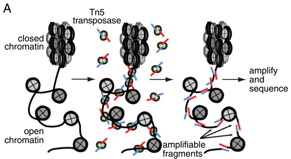
ATAC-seq overview (Buenrostro et al., 2015).
And the peaks look like the following figure.
ATAC-seq peaks (Tsompana and Buck, 2014)
And ATAC-seq can be used to:
- generate epigenomic profiles
- map accessible chromatin across tissues or conditions
- retrieve nucleosome positions
- identify important transcription factors
- generate occupancy profiles of TFs (footprinting)
Experimental design
See Buenrostro et al., 2015, ENCODE - ATAC-seq Data Standards and Prototype Processing Pipeline, and Harvard FAS Informatics - ATAC-seq Guidelines for details.
- two or more biological replicates
- each replicate has 25 million non-duplicate, non-mitochondrial aligned reads for single-end sequencing and 50 million for paired-ended sequencing
- typically, no need for “input”
- use as few PCR cycles as possible when constructing the library
- paired-end sequencing is preferred
Data analysis
Several useful pipelines.
- Harvard FAS Informatics - ATAC-seq Guidelines – clear and up-to-date.
- ENCODE - ATAC-seq Data Standards and Prototype Processing Pipeline
- Tobias Rausch - ATAC-seq analysis pipeline
- ENCODE ATAC-seq pipeline
- Parker Lab - ATAC-seq lab for BIOINF525
- Ferhat Ay Lab - ATAC-seq processing pipeline
- Rockefeller University, ATACseq in R
- 生物信息学生 R 入门教程 - 第五章 ATAC-seq数据分析 – in R.
The following pipeline includes several common analysis in ATAC-seq setting, from data trimming to peak calling. Some steps are optional, like merging BAMs.
Quality control
Just like analyzing other NGS data, quality control is needed for raw FASTQ, and there are many programs avaliable, such as Trimmomatic and Trim Galore.
Alignment and filter
The next step is to align reads to a reference genome. Two popular aligners are BWA and Bowtie2. I will use Bowtie2 (since it was used in many tutorals and papers).
1 | better alignment results are frequently achieved with --very-sensitive |
Then, the alignment results should be filtered.
Mitochondrial reads
Ref: Harvard FAS Informatics - ATAC-seq Guidelines
Since there are no ATAC-seq peaks of interest in the mitochondrial genome, these reads will only complicate the subsequent steps. Therefore, we recommend that they be removed from further analysis, via one of the following methods:
- Remove the mitochondrial genome from the reference genome before aligning the reads. In human/mouse genome builds, the mitochondrial genome is labeled ‘chrM’. That sequence can be deleted from the reference prior to building the genome indexes. The downside of this approach is that the alignment numbers will look much worse; all of the mitochondrial reads will count as unaligned.
- Remove the mitochondrial reads after alignment. A python script, creatively named removeChrom, is available in the ATAC-seq module to accomplish this.
Since the percentage of mtDNA-reads is a indicator of library quality, we usually remove mitochondrial reads after alignment. It is run as follows:
1 | samtools view -@ $PPN -h ${sample}.bam | grep -v chrM | samtools sort -@ $PPN -O bam -o ${sample}.rmChrM.bam |
PCR duplicates
Ref: Harvard FAS Informatics - ATAC-seq Guidelines
PCR duplicates are exact copies of DNA fragments that arise during PCR. Since they are artifacts of the library preparation procedure, they may interfere with the biological signal of interest. Therefore, they should be removed as part of the analysis pipeline.
One commonly used program for removing PCR duplicates is Picard’s
MarkDuplicates.
1 | {path2java} -XX:ParallelGCThreads=${PPN} -Djava.io.tmpdir=/tmp -jar ${path2picard} MarkDuplicates \ |
MarkDuplicates will add a FALG 1024 to duplicate reads, we can remove them using samtools:
1 | samtools view -h -b -F 1024 ${sample}.bam > ${sample}.rmDup.bam |
Non-unique alignments
Ref: Harvard FAS Informatics - ATAC-seq Guidelines
Some researchers choose to remove non-uniquely aligned reads, using the
-qparameter ofsamtools view.
Different genome aligners have varied implementation of mapping quality (MAPQ). See More madness with MAPQ scores (a.k.a. why bioinformaticians hate poor and incomplete software documentation). So, when using MAPQ to filter non-unique alignments, do check the MAPQ values of the aligner using.
For Bowtie2, people usually use MAPQ > 30.
1 | Remove multi-mapped reads (i.e. those with MAPQ < 30, using -q in SAMtools) |
Others
In the pipeline by ENCODE or some papers, the following reads were also removed (samtoolf flag 1796 or 1804).
- reads unmapped,
- not primary alignment
- reads failing platform
- duplicates
The remaining reads are so-called “properly mapped reads”.
1 | Remove reads unmapped, mate unmapped, not primary alignment, reads failing platform, duplicates (-F 1804) |
Merging BAMs (optional)
When several libraries were constructed for one experimental condition (aka. one experimental condition inlcuded several biological and/or technical replicates), one may want to merge different BAM files before calling peaks (e.g. merge BAM files from technical replicates, merge BAM files to get bigger read depth).
Considerations about “merge BAMs” or “merge peaks” have been discussed:
-
ChIP-Seq: Calling peaks with replicates
First, are these A) technical or B) biological replicates? That is, the same biological sample run several times with the same antibody (same lot also if polyclonal) protocol, or different biological samples run the same way with the same protocol?
If it is A it may be reasonable to merge them for some analyses, such as just annotating peaks. I would merge the bam alignment files and then do the calls versus merging the calls.
However, first you have analyze your replicates to check they they all perform the same. We did a lot of performance comparisons here: https://epigeneticsandchromatin.biomedcentral.com/articles/10.1186/s13072-016-0100-6
You can steal those ideas, especially using the ENCODE segmentation tracks if it’s human and they have tracks for something like your cell type. But just counting the reads in bins and then doing a correlation is pretty informative.
But even in our data, and we used a robot and do it a lot, one of our technical replicates behaved strangely. See supplemental figure S6.
If it is B, biological replicates, you almost certainly don’t want to merge them. You will lose your information about biological variance is present. If you are looking at something like differential peaks between conditions DESeq and really all reputable programs will want some sort of replicates, almost always biological. In general, if you want to compute a p value on anything you need separate replicates (not merged).
If you are just annotating peaks you don’t need a p value.
And merging BAM can be done using samtools.
1 | samtools merge -@ $PPN condition1.merged.bam sample1.bam sample2.bam sample3.bam |
Also, multiBamSummary in deepTools can be used to check the correlations between BAM files before merging.
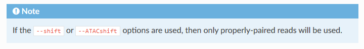
Shifting reads
In the first ATAC-seq paper (Buenrostro et al., 2013), all reads aligning to the + strand were offset by +4 bp, and all reads aligning to the – strand were offset −5 bp, since Tn5 transposase has been shown to bind as a dimer and insert two adaptors separated by 9 bp (Adey et al., 2010).
Ref: shifting reads bam for NucleoATAC?
However, for peak calling, shifting of reads is not likely very important, as it is a pretty minor adjustment and peaks are 100s of basepairs. The shifting is only crucial when doing things where the exact position of the insertion matters at single base resolution, e.g. TF motif footprinting.
Also, remember that not all TF footprinting tools need shifted reads. Some of them may do this internally, e.g. NucleoATAC.
But, how to adjust the reads alignment?
First, we could do this using bedtools and awk.
Ref: Shifting reads for ATAC-seq alignments
1 | the BAM file should be sorted by read name beforehand |
Or, we could do this using alignmentSieve.
1 | use --ATACshift |
We could also do this in R using ATACseqQC
1 | ## load the library |
Peak calling using MACS2
Ref: Biostars - ATACseq with STAR and macs2
You typically use the
--nomodeloption, as the shifting model of MACS does not really make sense for open chromation data. As you have probably paired-end data, also use the-f BAMPEoption. It forces MACS to pileup the real fragment length instead of an estimate, which maked sense imho, due to the quiet different fragment sizes that the library prep creates, also if you have paired-end why not make full use of it. Check reproducibility of the peaks between replicate samples, then rerun MACS with the merged bam file and feed the count matrix into DESeq2. Reference e.g. Corces et al 2016 Nat Genetics.
Ref: ATAC-seq settings · Issue #145 · taoliu/MACS
Liu Tao: If you followed original protocol for ATAC-Seq, you should get Paired-End reads. If so, I would suggest you just use
--format BAMPEto let MACS2 pileup the whole fragments in general. But if you want to focus on looking for where the ‘cutting sites’ are, then--nomodel --shift -100 --extsize 200should work.
Since paired-end sequencing is commonly used in ATAC-seq, so, we will tell MACS2 that the data is paired using the -f argument. By this way, MACS2 would only analyze properly mapped reads (as we get the bam after filtering above). The fragments are defined by the paired alignment, and there is no modeling or artificial extension.
1 | -f BAMPE, use paired-end information |
Creating browser tracks
If -B parameter was used when running macs2 callpeak, you would get bedGraph files together with narrowPeak files. Someone would use these bedGraph files to create browser tracks (e.g. ParkerLab - ATAC-seq lab for BIOINF545), while others say they look kind of weird (Biostars - How to compare bigwig tracks of two ATAC libraries). I do not know yet.
I would like to create bigWig files for visualizing using bamCoverage in deepTools. It provides several different ways to normalize the signal.
1 | bam to bigwig, normalize using 1x effective genome size |
Quality check
In processing ATAC-seq data, we would get several metrics to check the quality of data/libraries.
Ref:
Here is the standards used by ENCODE, and the detailed description of each term will be explained below.
")
Fragment/Insert size
Ref: Not A Rocket Scientist - ATAC-seq insert size plotting
One common QC for the data is to plot the fragment size density of your libraries. The successful construction of a ATAC library requires a proper pair of Tn5 transposase cutting events at the ends of DNA. In the nucleosome-free open chromatin regions, many molecules of Tn5 can kick in and chop the DNA into small pieces; around nucleosome-occupied regions, Tn5 can only access the linker regions. Therefore, in a normal ATAC-seq library, you should expect to see a sharp peak at the <100 bp region (open chromatin), and a peak at ~200bp region (mono-nucleosome), and other larger peaks (multi-nucleosomes). Examples from one of my data:
Regular scale:

Log scale:
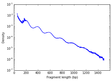
This clear nucleosome phasing pattern indicates a good quality of the experiment.
Different people probably have different way of plotting this using different codes, but making this plot can be simply achieved by a combination of one line of code and Excel. You don’t need some complicated scripts to do it at all.
samtools view ATAC_f2q30_sorted.bam | awk '$9>0' | cut -f 9 | sort | uniq -c | sort -b -k2,2n | sed -e 's/^[ \t]*//' > fragment_length_count.txt
See discussions here: Biostars - ATAC-seq fragment length distribution
%mitochondrial reads
High mitochondrial reads was a well-known problem, but in the latest ATAC-seq protocol (Omni-ATAC) this problem has been well addressed (Corces et al., 2017).
I guess in the future people will not care about this any more, and I keep this section in case.
Ref: Harvard FAS Informatics - ATAC-seq Guidelines
It is a well-known problem that ATAC-seq datasets usually contain a large percentage of reads that is derived from mitochondrial DNA (for example, see this discussion). Some have gone as far as using CRISPR to reduce mitochondrial contamination. The recently published Omni-ATAC method uses detergents to remove mitochondria and is likely to be more accessible for most researchers (but, do not follow their computational workflow).
The following code can be used to compute the percentage of mitochondrial reads.
Ref: Biostars - ATACseq alignment issues
1 | !/bin/bash |
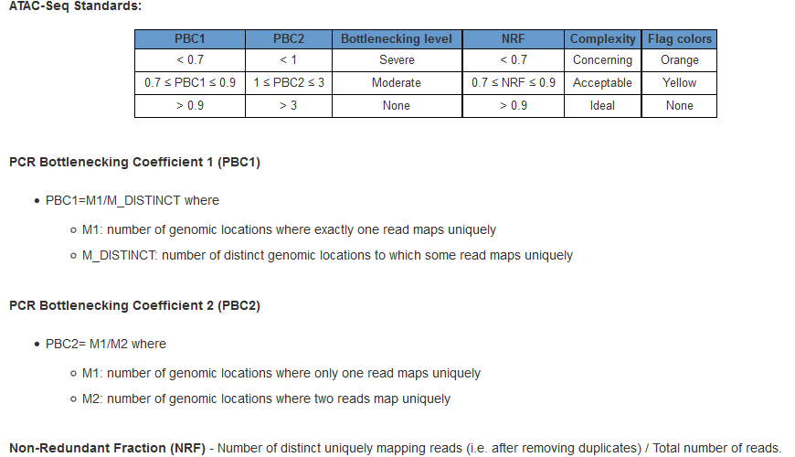
Library complexity
Ref: ENCODE - ATAC-seq Data Standards and Prototype Processing Pipeline
Library complexity is measured using the Non-Redundant Fraction (NRF) and PCR Bottlenecking Coefficients 1 and 2, or PBC1 and PBC2. The preferred values are as follows: NRF>0.9, PBC1>0.9, and PBC2>3.
The following code was from ENCODE ATAC-seq pipeline.
1 | the bam used here is sorted bam after duplicates marking |
Fraction of reads in peaks (FRiP)
Ref: ENCODE - Terms and Definitions
Fraction of reads in peaks (FRiP) - Fraction of all mapped reads that fall into the called peak regions, i.e. usable reads in significantly enriched peaks divided by all usable reads. In general, FRiP scores correlate positively with the number of regions. (Landt et al, Genome Research Sept. 2012, 22(9): 1813–1831)
Ref: Biostars - FRIP score ATAC-seq
In paired-end sequencing, we use the word fragment because the two reads that are produced always originate from the same DNA fragment and are therefore not independent of each other as reads from single-end sequencing would be. As FRiP comes from single-end ChIP-seq data, this is why they probably termed it reads. ATAC-seq is most commonly paired-end. You can use BEDtools for paired-end data but it requires more pre-processing of your data, that is why I use featureCounts, being faster and more convinient with plenty of customizable options. Choice is still yours. FRiP is probably not a very objective measure anyway, as it highly depends on how you prefilter your data, e.g. in terms of mapping quality, the definition of a properly-paired reads and the stringency of your peak calling (last sentence thinking aloud).
Ref: ENCODE - ATAC-seq Data Standards and Prototype Processing Pipeline
The fraction of reads in called peak regions (FRiP score) should be >0.3, though values greater than 0.2 are acceptable. For EN-TEx tissues (ENCODE GTEx tissue sample), FRiP scores will not be enforced as QC metric. TSS enrichment remains in place as a key signal to noise measure.
FRiP score can be calculated by samtools and bedtools:
1 | total reads |
While someone recommended to use featureCounts (https://www.biostars.org/p/337872/#337890), I found the results of featureCounts and intersectBed were close. So, I would like to use bedtools.
1 | samtools view -c ${sample}.bam |
Find more details in note: Calculate FRiP score.
Transcription start site (TSS) enrichment
Ref: ENCODE - ATAC-seq Data Standards and Prototype Processing Pipeline
Transcription start site (TSS) enrichment values are dependent on the reference files used; cutoff values for high quality data are listed in the table below.
Ref: ENCODE - Terms and Definitions
Transcription Start Site (TSS) Enrichment Score - The TSS enrichment calculation is a signal to noise calculation. The reads around a reference set of TSSs are collected to form an aggregate distribution of reads centered on the TSSs and extending to 1000 bp in either direction (for a total of 2000bp). This distribution is then normalized by taking the average read depth in the 100 bps at each of the end flanks of the distribution (for a total of 200bp of averaged data) and calculating a fold change at each position over that average read depth. This means that the flanks should start at 1, and if there is high read signal at transcription start sites (highly open regions of the genome) there should be an increase in signal up to a peak in the middle. We take the signal value at the center of the distribution after this normalization as our TSS enrichment metric. Used to evaluate ATAC-seq.
The following code was from ATAqC.
1 | import numpy as np |
Blacklist filtering for peaks
One may want to filter peaks using DAC Blacklisted Regions.
The following code was from ENCODE - ATAC-seq Data Standards and Prototype Processing Pipeline
1 | PEAK="${PREFIX}.narrowPeak" |
The 5th column of narroPeak file is integer score for display calculated as int(-10*log10qvalue). Since currently this value might be out of the [0-1000] range defined in UCSC Encode narrowPeak format, the awk code is to assign values greater than 1000 to 1000.
Merging peaks (optional)
One may want to merge peaks from different libraries or different samples.
Corces et al., 2016 used the following method to merge peaks, and I like their way:
To generate a non-redundant list of hematopoiesis- and cancer-related peaks, we first extended summits to 500-bp windows (±250 bp). We then ranked the 500-bp peaks by summit significance value (defined by MACS2) and chose a list of non-overlapping, maximally significant peaks.
We can do this by using BEDOPS (ref: Collapsing multiple BED files into a master list by signal)
1 | !/bin/bash |
Outreach
Well, then we complete the main upstream ATAC-seq data analysis. For downstream analysis, one may want to annotate peaks, find enriched motifs of TFs, compare peaks under different conditions and combine ATAC-seq data with other data types like RNA-seq etc.
Change log
- 20190103: create the note.
- 20190320: complete the note.
- 20190401: update the section of “Merging BAMs”. Add some discussions about “pooling replicates”